Julia set formed by f(z) = z2 + c where c = 0.687 + 0.312i
(click on any thumbnail image to view full size)
The infinite! No other question has ever moved so profoundly the spirit of man.
David Hilbert (1862-1943)
Julia set formed by f(z) = z2 + c where c = 0.687 + 0.312i
(click on any thumbnail image to view full size)
This presentation was prepared as the final assignment for the course Math 497 at the University of Washington, taught by James R. King, Ph.D in winter quarter 2000. This course dealt with selected topics in the behavior of complex numbers and functions. I was prompted to take this course (noncredit) by my long-standing though latent interest in the well-known fractal objects that are defined in complex planes, the Julia and Mandelbrot Sets, and am grateful to Professor King for offering it as an extension course. Along with the Feigenbaum (logistic) bifurcation diagram and the Hénon, Lorenz, and Rössler attractors, these fractal sets have come to epitomize the world of strange (i.e., fractal) attractors, and have captured the fancy and imagination of mathematicians and lay persons alike. It was my preference to attempt to survey the properties of Julia sets as broadly as possible rather than to focus solely on one or two subtopics (as might be more appropriate for the actual assignment), and this broad approach inevitably must result in some degree of superficiality. However, I have tried to avoid presenting a mere album of pretty images, and have tried to keep the discussion mainly at the mathematical level. Since the underlying mathematics is often abstruse and beyond my expertise, I have found it necessary to report some of the known properties of Julia sets without offering proof or further details.
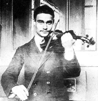
Julia sets are named after Gaston Julia. (He is depicted in the photo as a young man—one of the few photos available before he suffered a disfiguring facial wound in World War I). He was a French mathematician who discovered Julia sets and first explored their properties. He lived from 1893 to 1978 and his masterpiece on these sets was published in 1918 (Julia).
His interest apparently was piqued by the 1879 paper by Sir Arthur Cayley called "The Newton-Fourier Imaginary Problem" (Peitgen et al. 1992 p. 775). Cayley was studying the equation f(z) = z3 + c = 0, using the Newton-Fourier iterative method to seek the roots. Since there are three roots, he wondered if one could predict which of the three roots a given starting value of z would reach as a limit. He could not answer this question and commented that the problem "appears to present considerable difficulty" (Peitgen et al. 1992 p. 774). The solution, made apparent with modern computer iterative techniques, is that there are "basins of attraction" for each of the roots, such that a starting value of z falling in, for example, basin 1 will reach root 1 as the limit. But the shape of these basins is infinitely complex:
Here the three basins of attraction are colored green, yellow, and blue respectively, and are seen to be intricately interconnected. In fact, further magnification of this image, e.g., using the program WinFract.exe, demonstrates that the complexly interwoven pattern continues for all magnifications. Note that the diagram illustrates a somewhat more complex Julia set with underlying expression f(z) = z - ((z3 - 1)/3z2).
Julia did not live long enough to see a satisfactory visualization of the myriad and complex forms his sets take on—complexity in fact exceeding that exhibited by the Cayley problem. The creation of images of Julia sets and of other complex dynamical systems requires computer technology not readily available to him, and early attempts to depict them were very crude (Peitgen et al. 1992 p. 123).
Julia studied rational polynomial expressions of various degrees (e.g., z4 + z3/(z + 1) + z2/(z3 + 4z2 + 5)+ c), but in this presentation I will limit the discussion mostly to the family of sets generated by the special quadratic case form f(z) = z2 + c. Here z represents a variable of the form a+ib (a and b real numbers) which can take on all values in the complex plane. The quantity c also is defined as a complex number, but for any given Julia set, it is held constant (thus it is termed a parameter). In other words, there are an infinite number of Julia sets, each defined for a given value of c, though the ones with smaller values of c (i.e., |c| < ~ 2) are particularly interesting graphically.
Used once, the simple expression f(z) = z2 + c has little potential to create anything interesting—it is only by repeatedly
iterating it that the Julia set can be defined. When the output of the
expression f(z) is fed back into the expression as a new value of z, this is
called iteration, a type of feedback process. Thus, for any n:
zn+1 = f(z) = zn2 + c
and each new computed value of f(z) becomes the subsequent input value of z via the feedback loop.
Note that authors typically express purely real values of c such as -1+0i as "-1", and this can confuse the uninitiated who may not realize that c is still defined in the complex plane. For the special case where c=0+0i, the Julia set is simply a (nonfractal) circle with radius 1. A nice geometric explanation of the result of squaring a complex number and adding a complex constant to it is given at the Chaos Hypertextbook website (Elert 22.shtml). For any z, this transformation consists of a contraction (for |z|<1) or dilation (for |z|>1) resulting from multiplying by |z|, as well as a doubling of the polar angle (i.e., the argument) of z, and then a translation by c.
For any given starting value of z, say z0, there are two possibilities for what will happen to the iterated values of f(z) as n increases toward infinity: either f(z) can continue to grow without bounds or it will stay bounded. Points z0 in the complex plane that do not stay bounded with successive iterations of f(z) are said to be in the escape set Ec. All other points in the complex plane stay bounded as n is taken to infinity—they are termed prisoners and are said to be in the prisoner set Pc defined for a given c. All points must either be in one or the other set. The common boundary between the escape set and the prisoner set is called the Julia set Jc, defined for a particular value of c. The threshold radius r(c) = max(|c|, 2) provides a useful test criterion for computer implementation. If an orbit zk ever exceeds the threshold radius r(c), it is certain that the orbit will escape toward infinity and therefore the starting point is in the escape set (Peitgen et al. 1992 p. 794).
There seems to be a little definitional confusion in the literature as to whether the boundary points (i.e., the Julia set) are themselves part of the prisoner set, but this must be the case. The complex plane is divided solely into prisoner and escaping points, so the boundary points must belong to Pc since they cannot belong to Ec (otherwise they would escape under repetitive iterations, which is not the case). There are Julia sets (i.e., of boundary points) which do not enclose any interior prisoner points. Since Pc is by definition what remains of the complex plane after removing Ec, the boundary and prisoner points must coincide. An example of such a set is Jc for c=0+i (Peitgen et al. 1992 p. 798).
I have not seen this explicitly stated but suspect that there are no Julia sets having any escaping points which are completely surrounded by prisoner points.
As mentioned above, Julia sets can also be formed from higher degree and more complex expressions. The following are Julia sets for the iterated functions f(z) = z4 + c and f(z) = z5 + c, respectively:
The points of a Julia set (i.e., the boundary points) are "invariant" with respect to further iterations of f(z). Here, invariance does not imply that f(zj) = zj, but that, for any point zj belonging to the set Jc, f(zj) is also a member of Jc (Peitgen et al. 1992 p. 822).
Julia sets with purely real c (i.e., of the form c = a+0i) are reflection symmetric (that is, the part of the set below the real axis may be derived by reflecting the part above the real axis). Sets with complex c exhibit rotational symmetry—i.e., there is an axis passing through the origin which divides the set into parts which, when rotated 180 degrees, will coincide (Elert 22.shtml).
 A reflectionally symmetrical Julia set c = -1+0i |
 A rotationally symmetrical Julia set c = 0.3 + 0.6i |
Depending on the value of c selected, the resultant Julia set may be connected or disconnected—in fact, either totally connected or totally disconnected. There are several types of mathematical connectedness and I have not taken the opportunity to explore this topic in detail. In the case of Julia sets, I understand the type of connectedness referred to is "pathwise" connectedness, meaning that one can trace a path from a point in the set to other points in the set without leaving the set (Gagliardo). However, the type of connectedness referred to is less clear in Peitgen et al (1992 p. 803) and may not be pathwise. Connected Julia sets are "completely connected" as opposed to being merely "locally connected", a result shown independently by Julia and by Fatou (Gagliardo). Topologically, connected Julia sets are either equivalent to a severely deformed circle or to a curve with an infinite series of branches and sub-branches called a dendrite (e.g., the Julia set for c=0+i)" (Elert 22.shtml). Note that graphical displays of connected Julia sets often appear to demonstrate separate subsets even though they are in fact connected. When c is on the real axis (c = a+0i), the Julia sets are connected only for the x-interval [-2, 1/4] (Peitgen et al. 1992 p. 832).
Mandelbrot called disconnected Julia sets a "dust" of points (Mandelbrot p. 79), or "Fatou dust" (after Pierre Fatou 1878-1929) (Mandelbrot p. 182). This is a logical term, since a disconnected Julia set consists of individual points in the complex plane which, like sparsely sprinkled dust on a sheet, are not connected to any others. Another term used to describe a disconnected Julia set is Cantor dust (Peitgen et al. 1992 p. 798). The Cantor set of points is a totally disconnected set produced by successively dividing the line segment [0,1] in thirds and discarding the center segment yielding [0,1/3] and [2/3, 1], then repeating for each remaining line segment ad infinitum (Peitgen el al 1992 p. 68). The distribution of points in a disconnected Julia set qualitatively resembles the appearance of the more easily envisioned Cantor dust in that they are totally disconnected. Elert states "Disconnected sets are completely disconnected into a countably infinite assembly of isolated points. In addition, these points are arranged in dense groups such that any finite disk surrounding a point contains at least one other point in the set." (Elert 22.shtml).
The criterion which determines whether a Julia set is connected or disconnected will be discussed below with the Mandelbrot set.
The definition of fractal is inextricably connected to the concept of fractal dimension. We are all familiar with the topological dimension in describing the dimensionality of an object. A point has a topological dimension of 0, a curve or straight line a topological dimension of 1, a smooth surface a dimension of 2, and a smoothly demarcated solid object a dimension of 3. Even if curves, surfaces, or solids have rough or irregular edges, they may be deformed topologically to yield smooth objects with the stated topological dimensions. However, the fractal (non-topological) dimension of fractals (such as the Cantor dust of points or the Sierpinski gasket) incorporates the concept that their infinite ramifications in effect cover more of their Euclidean space than their topological dimension would suggest. For example, the well known Koch curve is a space-filling curve, a single line of infinite length and infinite angularity, which has topological dimension of 1 but a fractal dimension of log 4 / log 3 = c. 1.26. Speaking intuitively, it is able to cover more than the infinitesimal amount of the plane which a traditional one-dimensional curve can cover.
The exact definition of what constitutes a fractal seems to be undecided. Mandelbrot defined a fractal in 1977 as "a set in metric space for which the Hausdorff Besicovitch dimension D exceeds the topological dimension DT", but also stated that this rigorous definition should be considered tentative. He also offered a revised definition: "a set for which Frostman capacitary dimension > topological dimension" (Mandelbrot p. 361-2). In fact he believes that "one would do better without a definition." The topological dimension for the complex plane is simply 2. However, the choice of which of many fractal dimensional metrics is to be compared with the topological dimension is a controversial and complex subject.
Incidentally, it is often stated that a fractal has a fractional (nonintegral) dimension (the name fractal might seem to imply this), and this is usually the case, particularly regarding natural nonmathematically generated fractal objects. But some mathematical fractals have integer dimensions that exceed their topological dimensions. For example, Mandelbrot lists the path of Brownian motion (DT = 1, D = 2) and the Lebesque-Osgood monster surface (DT = 2, D = 3) (Mandelbrot p. 446-7).
Computer simulations verify the boundary of many of the Julia sets to be infinitely complex and never smooth regardless of the magnification, and thus such sets satisfy Mandelbrot's intended etymological root for fractal, i.e., having a fractured or broken contour— the Latin adjective fractus derives from the verb frangere meaning "to break" or create irregular fragments (Mandelbrot p. 4). The theoretical computation of the fractal dimension of a Julia set is apparently not a straightforward calculation and of course dependent on the dimension metric utilized and the parameter c. For instance, the 1992 textbook by Peitgen et al. does not include an estimate of the fractal dimension for Julia sets, though it does for the other strange (fractal) attractors described such as the Hénon attractor (D=1.28), Lorenz attractor (D=2.073), and Rössler attractor (c. 2.01-2.02). I have included citations by Saupe (cited in Peitgen et al 1992 p. 967) and by Mitsuhiro on this problem. The latter reported the Hausdorff dimension "H-dim" at the boundary of the M and Julia sets to be 2 (Mitsuhiro p. 225), but the details of this article are beyond my skill level. Elert used the Macintosh program Fractal Dimension Calculator (Bourke), which I have not been able to test. He calculated the empiric fractal dimension of a specific Julia set, that for c = -1+0i, and estimates the value at 1.16 (Elert 33.shtml). Obviously this result is at great variance with respect to Mitsuhiro's.
Fractals often exhibit self-similarity. Strict similarity is defined mathematically by Mandelbrot (Mandelbrot p. 349), paraphrased as follows: Given a real ratio parameter r, a positive integer N, and a bounded set S of points x = (x1, x2, x3, ..., xE) defined in a Euclidean space of dimension E , then S is self-similar if it is the union of N nonoverlapping subsets each of which is congruent to rS. Congruent means that they coincide, if necessary after a suitable rotation and displacement. This is readily observed in such regularly constructed and strictly self-similar objects as the Cantor set and the Koch curve (Peitgen et al. 1992 pp. 76, 204).
"[Suitably] selected fragments of a Julia set are strictly [self]-similar to the set as a whole." (Elert 23.shtml). In contrast, "fragments of the Mandelbrot [set] are only quasi-similar to the set as a whole. Furthermore, the motif of this quasi-self-similarity varies from one region to another and from one level of magnification to another." (Elert 23.shtml). Mandelbrot wished his own set, i.e., the "Mandelbrot Set", to be included as a fractal, so he introduced the concept of statistical self-similarity and self-affinity and other definitional extensions to include a broader range of objects that appear similar to the eye (Mandelbrot p. 350).
Other expected fractal properties, such as sensitivity, mixing, and periodicity are discussed below for Julia sets.
Any value of c is associated with fixed points for z, namely
the two (noniterative) solutions of the equation z2 -z + c = 0.
(This discussion of fixed points does not apply to the disconnected sets, about
which I
have found no information.) Taking as an example the connected set for c=-0.5+0.5i, the solutions to this
quadratic equation are given by
z = 1/2 ± (sqrt (1 - 4c))/2,
or
z = 1/2 ±
1/2sqrt((3 - 2i)), or
z1 = 1.4087-0.2751i
z2 = -0.4087+0.2751i.
For many values of c producing connected Julia sets (i.e., within the cardioid,
see below),
successive iterations of f(z) are found to converge to a single limiting z value = z2.
Moreover, the orbits of other starting points in the interior prisoner set
(i.e., not in the Julia set) when iterated converge to this fixed point.
Thus z2 is called an attracting fixed point and the interior prisoner
set lies in the basin of attraction for this point. (Incidentally, the
escape set of points for a Julia set may be said to lie in the basin of
attraction of the point at infinity.)
The other fixed point z1 behaves differently than z2. It is said to be a point on the Julia set and, provided sufficient calculation accuracy were available, iterations of this value are said to yield other points on the Julia set. (I tested this with Excel97, see julia.xls, and could not get it to work, presumably because of the need for exact accuracy.) Thus this fixed point is said to be a repelling fixed point. Peitgen et al elaborate that fixed points are repelling when the complex derivative at that point has absolute value >1, attracting when <1, and "indifferent" when =1 (Peitgen 1992 p. 822-823).
Objects like the Julia sets act as strange attractors, a term
coined by Ruelle and Takens and currently lacking a precise definition (Peitgen
1992 pp. 657, 671).
The word "strange" connotes the infinitely complex and self-similar fractal nature of
the attractor. For example, the Hénon attractor is comprised of an
infinite number of nearby but nonoverlapping curves, as are the Rössler and
Lorenz attractors. A Julia set is an attractor in the sense that
values of z belonging to Jc when further iterated continue to produce
other values lying in Jc. That is, the set seems to attract orbits
beginning in the set. Julia sets also act as attractors for the prisoner
and escape sets under the inverse transformation, see below. Like other chaotic systems
(Peitgen 1992 p. 536), Julia sets exhibit
(1) strong
sensitivity to initial conditions (i.e., the orbits of nearby points in Jc rapidly spread over the set with successive iterations), and
(2) strong mixing
inasmuch as the orbits of even a short
interval of adjacent points on the Julia Set will, with successive iterations,
spread out to quickly cover the entire Julia set (Peitgen et al 1992 p. 824).
The
third expected criterion which defines chaotic behavior is periodicity, and this
phenomenon is further described below.
The concept that a Julia acts as a strange attractor may be further illustrated as follows. Peitgen et al (1992 pp. 821 and 229-296) introduce the useful concept of what they call the "Multiple Copy Reduction Machine" (their name for an Iterated Function System). This is a sort of fancy and purely virtual photocopying machine which is capable of applying repeated nonlinear transformations to starting images according to a particular transformation formula. For Julia sets, they utilize transformation functions derived from the equation w = z2 + c to compute the "preimage" for any given image, namely w ±sqrt(w - c). A preimage P of an image I is the set of points which yields I when a transformation such as z2 + c is applied to P. It is therefore obtained by the inverse transformation of z2 + c, the transformation which is usually said to define Julia sets. When we iterate z2 + c for most connected Julia sets, the orbits of most starting points z0 in the z plane either tend toward the "fixed point" at infinity or toward the interior fixed point (exceptions include the Julia set points Jc, which are invariant). When the inverse expression for the transformation is iterated, the interior points of the prisoner set orbit outward and converge on the Julia set boundary, and similarly the exterior points in the escape set orbit inward and converge on the Julia set boundary. Therefore, all starting points of the plane are either already on or converge toward the Julia set in the limit under the inverse transformation. The Julia set seems in this sense to attract the orbits of all points of the z plane and thus may be termed an attractor. The iteration of the inverse transformation provides an alternative algorithm for computer generation of images of Julia sets.
Please note that it is my intention to focus on Julia sets, so that I will present only limited comments on the properties of the Mandelbrot set, primarily as it relates to Julia sets.
The Mandelbrot set M, discovered by Benoit B. Mandelbrot c. 1979, can be defined as the set of all values of the parameter c (Mandelbrot uses the character µ) for which the corresponding Julia sets are each connected, in fact totally connected. Alternatively, it can be defined as the set of values of c for which the orbits (successive iterations) of z0 = 0+0i remain bounded (Mandelbrot 183, Peitgen et al. 1992 p. 843). The point 0+0i is termed the critical point for Julia sets. This simple test, i.e., the boundedness of iterations of 0, thus determines whether a Julia set is connected, a result discovered independently by Julia and by Fatou (Gagliardo). The definition relating to iterations of 0 was the one Mandelbrot actually used in his initial explorations of M (Mandelbrot 183). M is a connected set, as shown by Douady and Hubbard (Peitgen et al. 1992 p. 849). However, this statement must apparently be qualified to "at least locally connected", since there are said to be an infinite number of points in M that are not currently known to be connected.
The definition of the prisoner set of a Julia set, defined as the Pc such that iterations of z —> z2 + c remains bounded, is similar to the second definition of the Mandelbrot set, where iterations of c —> c2 + c —> (c2 + c)2 + c . . . must remain bounded. However, although the points of the Mandelbrot set are defined in a complex plane, it has been emphasized that the Mandelbrot set lies in the plane of parameter values (c or µ) rather than the plane in which z values orbit (see for example Peitgen et al. 1992 p. 845). Elert provides the following further clarification: "One way to picture Mandelbrot and Julia sets is as complex ordered pairs (c, z) such that the mapping f: z —> z2 + c does not escape to infinity when iterated. Julia sets are slices parallel to the z-axis while the Mandelbrot set is a slice along the c-axis through the origin. As the coordinate system is complex, however, these 'axes' are actually planes. The Mandelbrot and Julia sets are therefore two-dimensional cross-sections through a four-dimensional parent set; the mother of all iterated quadratic mappings so to speak." (Elert 23.shtml) This author provided an interesting animation which demonstrated the transition between "successive slices through the four-dimensional mother set as we shift the cross-sectional plane from the z = 0 plane of the Mandelbrot set to the c = -1 plane of a particular Julia set (the San Marco Dragon)." (formerly at http://hypertextbook.com/chaos/movies/hybrid.mov). I must confess that I only dimly understand this concept.
Recall the threshold radius r(c) = max(|c|,2) described above: when an orbit yields any zk > r(c), this orbit will escape toward infinity. Note that r(c) can take on values greater than 2 when |c| > 2, though these sets will be disconnected. In contrast, the values of |c| for points in the Mandelbrot set must always be less than or equal to 2. On the real axis, the interval [-2, 0.25] consists entirely of points in M, and only for c=-2+0i can |c| = 2 (Peitgen et al. 1992 p. 845). To state also the obvious, for Julia sets having interior prisoner points, all points in the set lie on the boundary (i.e., Julia sets do not include interior points) whereas the points of the Mandelbrot include the interior points (i.e., the main cardioid and its buds often depicted in solid black).
M consists of a cardioid or heart-like main body extending on
the real axis from -0.75 to 0.25 and numerous "buds", the largest of
which extends to the left of -0.75, again on the real axis. Mandelbrot
terms these buds "atoms" (Mandelbrot 183). In the cardioid
region, one of the fixed points is attracting (and is the point to which
interior prisoner points converge) while the other is in the Julia
set and is repelling (Peitgen et al. 1992 p. 855). Peitgen et al. (1992) provide a pair
of equations parameterized on the parameter phi which generate this
cardioid:
x = 0.5cos(phi) -
0.25cos(2phi)
y = 0.5sin(phi)
- 0.25sin(2phi).
For example, the right margin of the cardioid is given for phi = 0 as
0.25+0i. When the parameter phi takes on values 2pi/k for integer values k
= 2,3,4,5,6,..., there is a bud extending outward from the cardioid. The
main or largest bud arises for phi = 2pi/2 (180°) and touches the cardioid at
only one point. This type of connection is apparently the case for other buds, but I am unsure
how general this rule is. This bud is a perfectly circular disk of
radius 0.25 centered at c=-1+0i (Peitgen et al. 1992 p. 862). Other buds
arises at phi = 2pi/3 = 120° and 2pi/4 = 90°. I have determined that the
parameter phi does not correspond to the usual polar angle for the complex
plane. For example, the values corresponding to phi = pi/2=90° are x =
0.25 and y = 0.5 whereas one would expect x to be 0 for complex argument =
90°. Moreover, the second largest bud (for which phi is 120° arises at
-0.125+0.64952i) visually appears to arise at a little more than 90° in the
complex plane with respect to the origin. Although Peitgen et al. (1992) do not
explicitly state this, it appears that buds also arise at values of phi = 2pi(1
+ n)/k for values of n = 0, 1, 2, ..., thus providing the matching buds by
symmetry. For example, the second largest bud, at phi = 120°, has a
matching counterpart at phi = 240°. I have calculated these budding
points and graphed them in an Excel97 spreadsheet MandelbrotCardioid.xls.
For any c lying within the largest bud (|1 + c| < 1/4), Peitgen et al. (1992 p. 863) demonstrate that the two fixed points of the Julia set are both repelling. One of the points iterates to infinity. The orbit of points starting near the other fixed point, after adequate iterations, stabilizes to an oscillation between two values (similar to the period-2 regime of the Feigenbaum bifurcation diagram). These "period" limit points do not correspond to either of the "fixed" points. Alligood et al (169) refer to the interior prisoner points of a typical period-3 Julia set as a basin of a "period-three sink". By comparison, the cardioid region of M corresponds to Julia sets having periodicity = 1 and in which the period-1 limiting point is the same as one of the fixed points. The disk of the largest bud is thus said to be the period-two disk. For example, when c=-1+0i, any prisoner point of the Julia set evolves to oscillate between 0+0i and 1+0i. This behavior can easily be confirmed in Excel (I have included the Excel97 worksheet julia.xls which can be used for this purpose). When c is other than -1 but in the period-2 disk, the period-2 alternating values are not usually integral. For example, for c = -0.75+0i, the orbit of the starting point -1+0i oscillates between about -0.531 and -0.468. All the prisoner points of this Julia set are attracted to this same period-2 orbit. I do not know if there are other values of c that lead to integral or rational Period 2 orbital values.
Similarly, the values of c within the next largest buds of M correspond to Julia sets with period-3 orbits for prisoner points, and other buds are associated with higher degrees of periodicity. This can be tested in the Excel application for example by selecting c=-0.12+0.74i, which lies in the large period 3 bud of M (arising at phi = 120°). After the orbit stabilizes (i.e., after 500 iterations or so), the orbital values are seen to cycle between -0.65306+0.56253i, -0.00995+0.00526i, and -0.11992+0.73989i. Other buds correspond to Julia sets with higher orbital periodicities. Peitgen et al. (1992 p. 866) state in essence the following: if two buds b1and b3 have periodicities p and q, then the periodicity of the largest bud b2 that is smaller than both b1 and b3 and which lies on the cardioid between them is equal to p + q.
Peitgen et al. (1992 p. 866) state that "indifferent" fixed points, which are neither attractive or repellent, arise for values of c right on the cardioid including at the touching points of buds. For some values of c corresponding to a parameter angle phi = 2(pi)m where m is irrational (such as -0.3905407802-0.5867879073i), the corresponding Julia prisoner set contains a disk called a Siegel disk (Peitgen et al. 1992 p. 868). The fixed point (-0.368684394 -0.337745165i in this case) is termed "irrationally indifferent" and the orbits of points near this fixed point within the Siegel disk rotate about the point but do not converge toward it. I have confirmed the behavior with the Excel97 simulation julia.xls.
I have prepared an Excel97 worksheet summarizing the fixed points, limiting period points, and the periodicity for selected values of c (points.xls) including several nonperiodic ones.
Some connected Julia sets consist of curves with no interior points. The most trivial example is c=-2+0i, for which the Julia set is a straight line [-2,0]. Other values of c such as c=0+i produce a dendritic pattern again with no interior points. Other Julia sets may contain both dendritic segments lacking interior points and regions with interior points, e.g., c = -1.77578 (Peitgen et al. 1992 p. 873).
The Mandelbrot set serves as a roadmap to or table of contents for the Julia sets (Peitgen et al. 1992 p. 855-895). To varying degrees, but in some cases quite striking, there is a correspondence or quasi-similarity between the appearance of portions of the Mandelbrot set and the Julia sets corresponding to the c values in that region of M. For example, at the so-called Misiurewicz points such as 0+i, the M and Jc sets become asymptotically similar as the degree of magnification increases and after suitable scaling and rotational adjustment (Peitgen et al. 1992 p. 887-8). This property of asymptotic similarity at Misiurewicz points was proven by Tan Lei (Peitgen et al. 1992 p. 889). A web-based interactive demonstration of quasi-similarity is found at the Julia and Mandelbrot Set Explorer website (Joyce; access restricted to academic proxy connection).
The mathematical behavior and graphical intricacies of the Julia sets provide fine examples of the fascinating world of strange attractors. I have enjoyed taking this opportunity to examine these sets.
All local images in this presentation have been created by the author using the FractInt clones WinFract.exe (see Griffin) or ChaosPro.exe 2.0 (see Pfingstl) unless otherwise noted, and modified or annotated in Adobe Photoshop as needed. They may be freely distributed and utilized as you see fit.


Julia sets for c = -1+0i and c=0.25+0i
Alligood KT, Sauer TD, Yorke JA. Chaos: An Introduction to Dynamical Systems. Springer-Verlag 1996. (A good overall mathematical review.)
Bourke P. "Fractal Dimension Calculator." (Macintosh software written Feb. 1993). Accessed 5 May 2000 <http://www.swin.edu.au/astronomy/pbourke/fractals/fracdim/>
Brin M [inferred]. "What is the Mandelbrot
Set?" Accessed 7 March 2000 <formerly at www.math.binghamton.edu/MATH/topics/mandel>
(Many full-sized color images with black and white thumbnail diagrams showing
the mapping of the M set to Julia sets.)
Cayley A. "The Newton-Fourier Imaginary
Problem." Amer. J. Math. 2, 1879 92
(Cited
in Peitgen et al 1992 p. 775)
Elert G. The Chaos Hypertextbook: Strange and
Complex. Accessed 5 March 2000 <http://hypertextbook.com/chaos/>.
(This site provides a good list of available Macintosh-oriented software for
generating fractals.)
Pfingstl M. "ChaosPro v. 2.0." Accessed 6
March 2000 (former URL http://home.att.net/~Paul.N.Lee/ChaosPro.HTML)
(This is a 32-bit updated version of FractInt.exe which appears to work quite
well but does not have all the choices of WinFract.exe.)
Gagliardo M. "The Julia Sets and Other Fractals." Accessed 7 March 2000, URL formerly http://rene.ma.utexas.edu/users/mgags/julia.html
Griffin N. "GETTING FRACTINT." Windows
version 18.21. Accessed 5 March 2000 formerly at http://spanky.triumf.ca/www/fractint/getting.html
(This site provides links to obtain the fractal generating software FractInt.exe
for DOS and WinFract.exe for 16-bit Windows.)
Griffin N. "WELCOME to the Fractint WWW page." Accessed 5 March 2000 formerly at http://spanky.triumf.ca/www/fractint/fractint.html
Joyce DE. "Julia and Mandelbrot Set Explorer." Accessed 6 March 2000 <http://aleph0.clarku.edu/~djoyce/julia/explorer.html>.
Julia G. "Mémoire sur l'itération des fonctions
rationnelles." Journal de Math. Pure et Appl. 8 (1918) 47-245.
Republished in Hervé M (ed.) Oeuvres de Gaston Julia: Vol. I. Gauthiers-Villars 1968 121-333.
(This is Julia's original description of Julia
Sets.)
Mandelbrot BB. The Fractal Geometry of Nature
(Updated and Augmented). W. H. Freeman and Co. 1983 (Revised edition of Fractals c. 1977).
(The mother of all works in the computer era on fractals and strange attractors
but nearly incomprehensible.)
"The Math Forum." Accessed 19 February 2006 <http://mathforum.org/>.
(An excellent starting place for obtaining mathematical information and
materials at all levels.)
Mitsuhiro S. "The Hausdorff Dimension of the Boundary of the Mandelbrot Set and Julia Sets." Ann. Math. 147 (1998) No. 2 225-267.
Peitgen H, Jurgens H, and Saupe D. Chaos
and Fractals: New Frontiers of Science. Springer-Verlag, 1992.
(A superb and detailed textbook discussing many aspects of fractals and chaos,
including the Julia and Mandelbrot sets.)
Peitgen HO and Richter PH. The Beauty
of Fractals: Images of Complex Dynamical Systems. Springer-Verlag
1986.
(An often quoted work which I have not had the chance to review in detail.)
Saupe D. "Efficient Computation of Julia Sets and Their Fractal Dimension." Physica D28 (1987) 358-370 [cited in Peitgen et al. 967].

Page mcgoodwin.net/julia/juliajewels.html
Created by Michael McGoodwin
Last update: 28 October 2022
![]()